I’m a big fan of Doctor Who, so when the new series came out earlier this year I was inspired to do some exploratory analysis of scripts from the show. Doctor Who is about a time-travelling alien (the Doctor) who explores the universe with a series of companions, generally getting himself into lots of trouble and saving the world a few times along the way. The Doctor has the ability to regenerate instead of dying, which means that the show can fairly gracefully replace the actor playing him. The current Doctor is the thirteenth overall and the fifth since the show relaunched in 2005. The characters the Doctor travels with also change every so often. This means the show has an interesting mix of recurring and non-recurring characers, with the Doctor the one fixed character.
Scripts of the show are available on this site, so this project gave me the chance to practice scraping and cleaning data. While that process is not going to be the focus of this post, you can see the script I used for this in my GitLab. For this analysis, I’ll be focusing on episodes from 2005 onwards. This gives me eleven seasons of scripts to worth with (actually, eleven and a bit, since the current season is still running).
Initial exploration of the script data
I’ve processed the scripts into a ‘tidy’ form, which makes them easier to work with as all the information I need is included in each row. I have a different row for each line of dialogue that includes the name of the episode, the scene number, the character speaking, and which doctor is in the episode. Adding the doctor column is important because the doctor almost always appears in the scripts as just ‘DOCTOR’, and at some point I may want to look at differences between Doctors. The resulting data.table has over 75000 lines and includes over 1000 different characters.
We can now start to explore the data and form some questions.
library(magrittr)
library(treemap)
dt_scripts[, .N, by = "character"][!(character %like% "\\+") & N > 200] %>%
treemap(index = "character",
vSize = "N",
type = "index",
palette = "Spectral",
title = "Which characters have the most lines?",
fontface.labels = 2)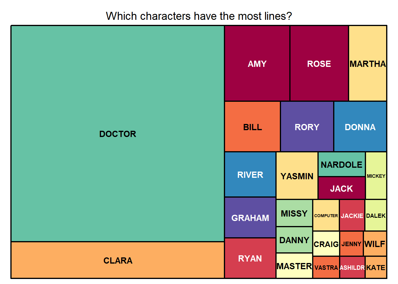 Here I’ve used a treemap to get a sense of the number of lines spoken by character across all episodes (only characters with at least 200 lines are shown). Unsurprisingly, the Doctor has by far the most lines. Companions also have quite a lot of lines, and we also see other recurring characters who are friends (like Vastra and Jenny) or enemies (Dalek, the Master, and Missy). These 27 characters account for over 60% of all the lines spoken.
library(ggplot2)

dt_scripts[, .N, by = episode] %>%
    ggplot() +
    geom_histogram(aes(N), binwidth = 20, fill = "midnightblue") +
    theme_classic() +
    scale_y_continuous(expand = c(0, 0)) +
    xlab("Number of lines") +
    ylab("Number of episodes") +
    ggtitle("How many lines are there in each episode?") +
    theme(plot.title = element_text(hjust = 0.5))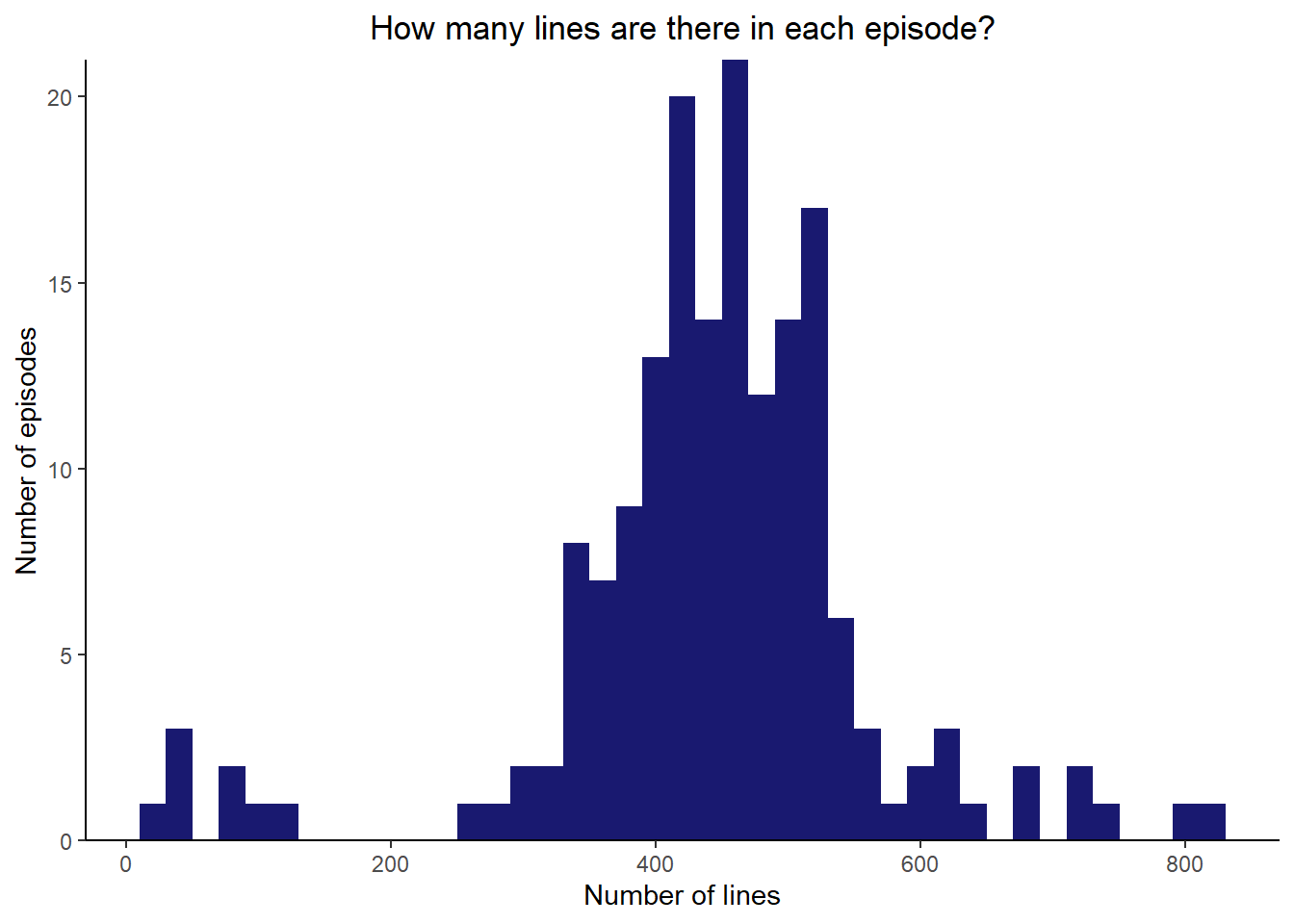
I’ve also made a histogram showing the number of lines per episode, in part to get a sense of whether my scraping and cleaning of the scripts might have failed. This could manifest in some oddly long or oddly short episodes. There are a small number of episodes with < 150 lines that look a bit suspicious to me, but on inspection these all turn out to be special episodes that are very short.
Visualising interactions between characters
I would like to find a way to visualise the relationships between characters. One proxy for interactions is the number of scenes that characters both appear in, which I can get from my dataset. I’m going to use the package igraph to display these relationships, with vertices representing characters and edges representing scenes both appear in.
This isn’t a perfect approach, as two characters appearing in a scene doesn’t necessarily mean they interact (for example, one could leave before the other enters or one could be unaware the other is there). That said, this is a fairly straightforward way to get a sense of character interactions and I can use my domain knowledge of Doctor Who to figure out if the results make sense or not. Another potential problem with this approach is that sometimes different characters have the same name. For example, daleks often appear in the script simply as ‘DALEK’, so all the lines spoken by daleks end up being attributed to one character. This is also a problem for Clara’s boyfriend Danny, as there is a different character called Danny in an episode in an earlier season.
Note that here I’m using igraph in a very simple way to visualise the relationships on the show, but you can use graphs to tackle much more complex questions. For example, graphs can be used to model social networks, where you can use them to answer questions about which people are most central to the network and different ways people can be connected.
I’ll begin by creating a data.table showing the number of interactions between different pairs of characters that will be the edges of my graph. I’m only going to visualise the top 27 characters (by total number of lines), as with many more this will get very messy to plot.
top_27 <- dt_scripts[,
                     .N, by = character
                     ][order(-N)
                       ][
                         1:27, character
                         ]
dt_scripts_graph <- dt_scripts[character %in% top_27]
dt_scripts_graph[character %like% "DOCTOR", character := "DOCTOR"]
dt_scripts_graph[character %like% "YASMIN", character := "YAZ"]
dt_scripts_graph <- unique(dt_scripts_graph,
                           by = c("character", "episode", "scene"))
dt_scripts_graph[, `:=`(doctor = NULL, dialogue = NULL)]
dt_scripts_graph[, character := stringr::str_to_title(character)]

dt_linecount <- dt_scripts_graph[, .N , by = character]
character_linecounts <- dt_linecount$N
names(character_linecounts) <- dt_linecount$character

dt_edges <- dt_scripts_graph[dt_scripts_graph,
                          on = .(scene = scene, episode = episode),
                                 allow.cartesian = TRUE][
                              character != i.character
                          ][
                              character < i.character
                          ][
                              , .(count = .N), by = .(character, i.character)
                          ]

dt_edges[order(-count)]
## character i.character count
## 1: Clara Doctor 522
## 2: Amy Doctor 409
## 3: Doctor Rose 322
## 4: Amy Rory 263
## 5: Doctor Rory 247
## ---
## 164: Donna Missy 1
## 165: Jack Missy 1
## 166: Jenny Missy 1
## 167: Amy Missy 1
## 168: Dalek Graham 1Even without plotting the graph, we already get some sense of what the most important interactions are going to be. Almost all of the most frequent interactions are the Doctor interacting with companions.
Now we can visualise these interactions. I’m also incorporating some extra information (such as total number of lines spoken by each character and their role) that I can add to the final visualisation. igraph allows you to make graphs in a number of different ways, but here I’ll use my data.table of edges.
library(igraph)

character_graph <- graph_from_edgelist(as.matrix(dt_edges[, 1:2]),
                                       directed = FALSE)

E(character_graph)$weight <- dt_edges$count
E(character_graph)$width <- log2(E(character_graph)$weight) / 2

V(character_graph)[name == "Doctor"]$role <- "doctor"
companions <- c("Clara", "Amy", "Rose", "Martha", "Bill",
                "Donna", "Yaz", "Ryan", "Graham")
V(character_graph)[name %in% companions]$role <- "companion"
V(character_graph)[is.na(role)]$role <- "other"
role_colours <- c(doctor = "#6c6ca4", companion = "#73aa73", other = "#bf7373")
V(character_graph)$color <- role_colours[V(character_graph)$role]
V(character_graph)$line_count <- character_linecounts[V(character_graph)$name]
V(character_graph)$names <- stringr::str_to_title(names(V(character_graph)))
plot(character_graph,
vertex.color = adjustcolor(V(character_graph)$color),
vertex.label.color = "black",
vertex.label.family="sans",
vertex.size = log2(V(character_graph)$line_count) * 1.2,
vertex.frame.color = NA,
layout = layout_with_fr(character_graph),
main = "Interactions between characters on Doctor Who",
)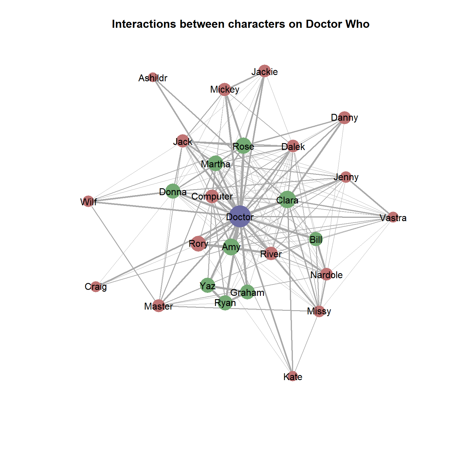
The resulting graph conveys a lot of information rather succinctly. A line between two characters indicates that those characters are in at least one scene together. The thickness of the lines between characters is proportional to the number of scenes both occur in, the size of the vertex represents the total number of lines for that character, and the colours indicate the character’s role in the show.
We can easily see the centrality of the Doctor to the show, as he has interactions with all other characters and also has the most lines. The Doctor interacts most frequently with companions, whereas other characters are more peripheral. This makes sense given that that the show focuses on the Doctor’s travels with various companions. We can also see connections between characters such as Rose, Mickey and Jackie that reflect their relationships that are independent of the Doctor.
Preparing the script dataset for textual analysis with quanteda
As this is a text-heavy dataset, one of the things I’m most interested in is performing a textual analysis. R has a lot of packages that can be used for this purpose, but here I’ll be using quanteda.
The first step in using quanteda is to create a corpus. A corpus is simply a collection of texts. What you define as a text depends on your dataset and kind of analysis you want to do, though it’s worth noting that once you have a corpus, you can then reshape it to break it apart into paragraphs or sentences. A corpus can also have associated document-level variables (docvars), which may be necessary for your analysis. In this case I’ll initially be treating each line as a text, which will result in an enormous corpus. Each line will have document-level variables such as the character who speaks the line and the episode the line is from. It could also make sense to aggregate by episode, depending on what you want to do. I’m initially interested in the differences between characters, so combining dialogue from different characters by episode doesn’t really make sense here.
library(quanteda)
dt_scripts[character == "DOCTOR", character := paste("DOCTOR", doctor)]
corpus_scripts <- corpus(dt_scripts, text_field = "dialogue")
Here I’ve also changed the DOCTOR to DOCTOR {number} in the character column so I can distinguish dialogue from different Doctors.
Aside from the corpus, the two other main types of objects you’ll work with in quanteda are tokens and document feature matrices (DFMs). Tokens are essentially just words (or groups of words), though there’s often a lot of filtering and manipulation that goes on in going from your text to tokens. Once you tokenise, the order of the words in your text is lost.
tokens_scripts <- corpus_scripts %>%
    tokens(
        remove_numbers = TRUE,
        remove_punct = TRUE,
        remove_hyphens = TRUE,
        include_docvars = TRUE,
        remove_symbols = TRUE
        ) %>%
    tokens_wordstem()
Here I have created tokens from my corpus. Most of the options I’ve chosen speak for themselves, such as removing numbers, punctuation, hyphens, and symbols. I’ve also opted to keep the docvars associated with each text/line.
The use of tokens_wordstem() requires some explanation. Stemming shortens words to their stem; for example, the word ‘running’ becomes ‘run’ and ‘dogs’ becomes ‘dog’. This can be a useful step, since these pairs of words involve the same basic concept and so it probably doesn’t make sense to look at them separately. An alternative to stemming is lemmatization. Lemmatization goes a little further than stemming and can change a word beyond just shortening it. For example, the word ‘went’ would become ‘go’. Both approaches will reduce the total number of tokens, but lemmatization will generally reduce it more.
In this analysis I’ve opted to use stemming instead of lemmatization, in part because it’s a more conservative approach. For example, Rose is the name of one of the Doctor’s companions and so her name appears frequently in the dialogue. However, ‘rose’ is also the past tense of ‘rise’, so if I lemmatize the name ‘Rose’ will be changed to ‘rise’. In this context this would be very confusing and would mess up my analysis. While lemmatization can be very powerful, it’s important to bear things like this in mind and sanity check your findings to uncover anything weird like this that might distort your results.
Once you have tokens, the next step is to make a document frequency matrix (DFM). You can actually do this directly from a corpus object, but this givens you less control over the tokenisation.
dfm_all <- dfm(tokens_scripts,
               tolower = TRUE,
               remove = stopwords(source = "smart"))
The document frequency matrix (DFM) is a huge matrix in which each column is a different token and each row is a text. The DFM has the count of each token for each text. The docvars from the corpus and token objects carry through, so the character and episode information is still there. This means if I decide I want to filter out dialogue from some characters or aggregate by episode, I can do this directly from my existing DFM rather than have to go back to the corpus object. The DFM will be the object I will most often work with for subsequent analysis. It will often require some filtering or aggregation to answer specific questions.
Here I’ve chosen to remove stop words, which are commonly occurring works like ‘am’ and “there” that are so frequent that including them doesn’t add anything to the analysis.
Identifying differences between characters based on their dialogue
I’m interested in understanding how different the dialogue of various characters is. I’ll restrict this analysis to the top 15 characters in the show. This means subsetting my existing DFM and grouping by character. The quanteda library has a function topfeatures() that shows you the tokens with the highest counts in the DFM for each row (in this case, for each character). I can then reformat the output to view it more easily.
top_15  <- dt_scripts[ , .N , by = character][order(-N)][1:15, character]
dfm_top <- dfm_all %>%
    dfm_subset(character %in% top_15) %>%
    dfm_group(groups = "character")

features_top15 <- topfeatures(dfm_top, 10, group = "character")
dt_features <- as.data.table(as.data.frame(sapply(features_top15,
function(x) names(x))))| AMY | BILL | CLARA | DOCTOR 10 | DOCTOR 11 | DOCTOR 12 | DOCTOR 13 | DOCTOR 9 | DONNA | GRAHAM | MARTHA | RIVER | RORY | ROSE | RYAN |
|---|---|---|---|---|---|---|---|---|---|---|---|---|---|---|
| doctor | yeah | doctor | time | time | you’r | you’r | you’r | doctor | yeah | doctor | doctor | doctor | doctor | yeah |
| rori | doctor | whi | you’r | you’r | time | whi | rose | you’r | doc | you’r | time | ami | yeah | hey |
| yeah | whi | you’r | yeah | ami | clara | time | time | yeah | you’r | yeah | you’r | yeah | you’r | we’r |
| whi | you’r | yeah | back | whi | whi | back | thing | whi | ryan | time | love | er | mum | doctor |
| you’r | er | sorri | thing | back | veri | we’r | back | back | we’r | thing | back | you’r | time | thing |
| time | time | time | good | yeah | becaus | veri | you’v | thing | thing | sorri | whi | sorri | back | you’r |
| happen | thing | er | sorri | good | thing | thing | yeah | becaus | grace | back | man | time | thing | yaz |
| becaus | someth | realli | whi | thing | they’r | work | good | time | er | someth | they’r | whi | happen | happen |
| pleas | they’r | thing | stop | becaus | good | they’r | world | someth | hey | we’r | kill | back | whi | back |
| someth | peopl | happen | you’v | sorri | back | yaz | human | we’r | mate | you’v | die | happen | someth | er |
While this is a good start, we can start to see some problems with this approach. For a start, we can see that the words ‘doctor’ and ‘time’ are very highly ranked for many of the characters. This tells us that these are commonly occurring words regardless of character, which is good to know but not very interesting. Secondly, there are a lot of character names. While this can be interesting to see, including character names in this kind of comparison can be misleading. This is because the names a character uses in speech are not really related to how they talk, but rather who they’re with. Incidentally, you can also see the effects of the stemming in these results, which leaves some words looking a bit odd (such as ‘sorri’). Some character names have also been mangled a bit.
To try to identify words that are more specific to each character, we’ll use a statistic called TF-IDF (term frequency - inverse document frequency). This is a measure of how frequently a word is used in one document (in this case, a character) relative to how frequently it’s used generally (by all characters). A term with a very high TF-IDF will be used very frequently by one character and almost never by others. Ranking by TF-IDF will give us a better idea of what is distinctive about each character’s dialogue. I will also filter out character names (and stemmed variants of character names, where possible), since the presence of those tells us more about who a character spends time with than about their language choices.
names <- unique(dt_scripts$character)
names_stemmed <- tokens(names) %>% tokens_wordstem()

dfm_top_filtered <- dfm_top %>%
    dfm_remove(names) %>%
    dfm_remove(names_stemmed) %>%
    dfm_tfidf()

features_top15 <- topfeatures(dfm_top_filtered, 10, group = "character")
dt_features <- as.data.table(as.data.frame(sapply(features_top15,
function(x) names(x))))| AMY | BILL | CLARA | DOCTOR 10 | DOCTOR 11 | DOCTOR 12 | DOCTOR 13 | DOCTOR 9 | DONNA | GRAHAM | MARTHA | RIVER | RORY | ROSE | RYAN |
|---|---|---|---|---|---|---|---|---|---|---|---|---|---|---|
| angel | nardol | pink | viperox | pond | nardol | yaz | satellit | temp | doc | indigo | sweeti | jennif | what’r | yaz |
| pond | puddl | oswald | reinett | angel | vardi | pting | narrow | binari | yaz | shakespear | ramon | nurs | wilson | nan |
| cube | ars | souffl | allon | georg | oswald | kerblam | rift | gramp | cockl | annalis | spoiler | leadworth | tyler | logan |
| raggedi | sutcliff | gallifrey | wormhol | madg | pott | praxeus | nanogen | lanc | poli | jone | angel | nephew | shareen | sire |
| william | lectur | porridg | racnoss | cube | hybrid | resus | charl | clement | cos | osterhagen | aplan | doorknob | isolus | reload |
| melodi | um | maisi | infostamp | sophi | bank | ux | tyler | chiswick | nan | dalekanium | archaeologist | beard | moonlight | hann |
| pregnant | portion | franni | jone | dear | karabraxo | shaw | chula | dumbo | steve | arr | pandorica | drove | union | sinclair |
| mel | defect | blackpool | adelaid | gillyflow | gemston | orb | fantast | chaplin | grandson | mast | diamond | ma’am | jacki | luther |
| paisley | pott | muh | void | wifi | pe | dreg | what’r | hotter | sire | infinit | dear | astronaut | danc | cos |
| petrichor | verita | moat | torchwood | snow | rob | cos | calcium | neri | son | sir | darillium | attention | anymor | bike |
This is a much more interesting list, and it tells us a lot more about differences between the characters. For example, looking at River’s top-ranked terms we see ‘sweetie’, ‘archaeologist’ and ‘spoiler’, which are terms that I certainly associate with her. There are still some names appearing such as “williams” (Rory’s last name), but this is an improvement over the initial list.
Examining the relationship between the Doctor’s sentiment and overall episode sentiment
Sentiment analysis is often incorporated into text mining and analysis. This involves attempting to identify emotions associated with a particular text. Here I’m use the library sentimentr, since unlike many other libraries that can be used for sentiment analysis it takes into account valence shifters. This means that instead of detecting the word ‘good’ in a sentence and concluding that the sentiment is positive, it can take into account whether this is part of the phrase ‘not good’ and thereby has a negative sentiment. sentimentr can also identify emotions and profanity, which can also be interesting to look at though I don’t here.
I’ll first get the average sentiment score for every line of dialogue and look at the highest and lowest ranked to get some sense of how this works.
library(sentimentr)

dt_sentiment_short <- with(dt_scripts,
                           sentiment_by(
                             get_sentences(dialogue),
                             list(character, episode_num,
                                  episode, scene, dialogue)
                           ))

dt_sentiment_short[order(ave_sentiment)] %>% head()
## character episode_num episode scene
## 1: VASTRA 114 Deep Breath 11
## 2: DOCTOR 10 55 Midnight 19
## 3: DOCTOR 9 10 The Doctor Dances 3
## 4: DOCTOR 12 139 The Husbands of River Song 4
## 5: DANNY 123 In the Forest of the Night 36
## 6: DONNA 54 Forest of the Dead 18
## dialogue word_count sd ave_sentiment
## 1: I don't know, but I fear devilment. 7 NA -1.488235
## 2: Knock, knock. 2 NA -1.414214
## 3: I wish. 2 NA -1.414214
## 4: Slash murderer slash thief. 4 NA -1.400000
## 5: You're worrying too much. 4 NA -1.375000
## 6: Sorry, but you're dead. 4 NA -1.375000dt_sentiment_short[order(ave_sentiment)] %>% tail()## character episode_num episode scene
## 1: DOCTOR 11 73 Cold Blood 21
## 2: RIVER 92 The Wedding of River Song 23
## 3: DOCTOR 10 112 The Day of the Doctor 14
## 4: PHARMACIST 1 33 Gridlock 5
## 5: RORY 76 The Pandorica Opens 16
## 6: DOCTOR 10 50 The Poison Sky 105
## dialogue word_count
## 1: Not to interrupt, but just a quick reminder to stay calm. 11
## 2: Please, my love, please, please just run! 7
## 3: Whoa, whoa, whoa, whoa, whoa. Oh, very clever. 8
## 4: Happy, Happy, lovely happy Happy! 5
## 5: Whoa, whoa, whoa. 3
## 6: Please, please, please, please, please, please, please. 7
## sd ave_sentiment
## 1: NA 1.413334
## 2: NA 1.417367
## 3: 1.030004 1.507745
## 4: NA 1.677051
## 5: NA 1.732051
## 6: NA 2.645751Amongst the examples of dialogue with the lowest sentiment scores are “I don’t know, but I fear devilment”, “Sorry, but you’re dead”, and “Slash murderer slash thief”, which do seem solidly negative. Surprisingly, we also have “knock, knock” and “I wish”.
Similarly, the dialogue with highest sentiment scores includes “Whoa, whoa, whoa, whoa, whoa. Oh, very clever” and “Happy, Happy, lovely happy Happy!, but also”Please, my love, please, please just run!" and “Not to interrupt, but just a quick reminder to stay calm”.
Now I’m going to look at sentiment scores between Doctors to identify possible differences.
library(ggbeeswarm)
dt_sentiment <- with(dt_scripts,
sentiment_by(
get_sentences(dialogue),
list(character, episode_num, episode)))
dt_sentiment <- dt_sentiment[word_count > 50]
dt_doctors <- dt_sentiment[character %in% paste("DOCTOR", 9:13)]
dt_doctors[, character := factor(character, levels = paste("DOCTOR", 9:13))]
ggplot(dt_doctors, aes(character, ave_sentiment)) +
geom_beeswarm(aes(colour = character)) +
stat_summary(fun.y = "median", fun.ymax = "median", fun.ymin = "median",
geom = "crossbar",
width = 0.3) +
scale_color_viridis_d(end = 0.9) +
theme_classic() +
ggtitle("How does average sentiment vary by Doctor?") +
ylab("Average sentiment") +
theme(plot.title = element_text(hjust = 0.5),
legend.position = "none",
axis.title.x = element_blank())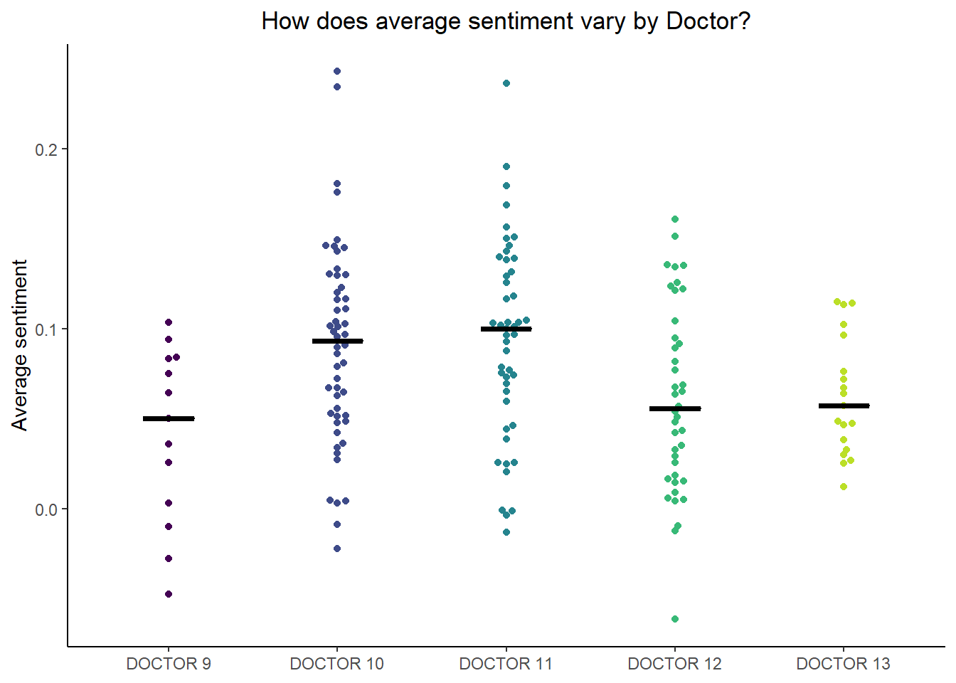 This beeswarm plot shows the average sentiment for each episode for each Doctor. I’ve excluded instances where the Doctor has fewer than 50 words in an episode, since in those cases the averages tend to be very high or very low.
There don’t seem to be large overall differences between Doctors, though Doctors 10 and 11 are a little cheerier than the others.
We can identify the episodes where the average sentiment for the Doctor is highest and lowest.
dt_doctors[which.min(ave_sentiment)]## character episode_num episode word_count sd ave_sentiment
## 1: DOCTOR 12 137 Heaven Sent 2587 0.2358146 -0.06130917dt_doctors[which.max(ave_sentiment)]## character episode_num episode word_count sd ave_sentiment
## 1: DOCTOR 10 56 Turn Left 171 0.2484174 0.2429945The episode with the lowest average sentiment is Heaven Sent, which is the episode after Clara dies. This makes sense, as it is a fairly dark episode. Surprisingly though, Turn Left is the episode with the highest average sentiment. Turn Left is about a dystopian alternative reality, so it’s not a particularly happy episode. It’s appearance here could be because this analysis focuses only on the Doctor’s dialogue, and since the episode actually focuses on Donna we don’t capture the overall tone of the episode. Indeed, the Doctor has only 171 words.
How does average sentiment per episode compare to sentiment of the Doctor’s dialogue only? Are Doctors 10 and 11 simply more chipper than the other because the episodes they appear in are overall cheerier? One way to approach this is by examining the relationship between the average sentiment of the Doctor’s dialogue and that of all other dialogue.
There are several possibilities for how the Doctor’s mood or sentiment in an episode could relate to the overall mood of the episode (as reflected in dialogue):
- The sentiment of the Doctor’s dialogue is not strongly related to that of others. This would suggest that the differences we see in the sentiment scores of different Doctors are due mostly to differences in personality
- The Doctor’s mood drives of the overall mood of the episode. That is, a happy Doctor leads to other characters’ dialogue also being more cheerful
- The Doctor’s mood is mainly influenced by the circumstances and tone of the episode
In the first case, we should see only a weak correlation between the sentiment of the Doctor’s dialogue and that of other characters. However, the final two cases will be difficult to distinguish. In both cases, we would see a strong correlation but we would not necessarily be able to say why this occurs.
library(ggpubr)

dt_sentiment_nodoc <- with(dt_scripts[!(character %like% "DOCTOR")],
                             sentiment_by(
                               get_sentences(dialogue),
                               list(episode_num, episode, doctor)))

dt_sentiment_episode_doctor <- dt_sentiment_nodoc[
  dt_doctors, on = "episode_num"
  ][
    , doctor := factor(paste("DOCTOR", doctor), levels = paste("DOCTOR", 9:13))
    ]

ggplot(dt_sentiment_episode_doctor, aes(ave_sentiment, i.ave_sentiment)) +
  geom_point(aes(color  = doctor)) +
  geom_smooth(method = "lm", se = FALSE, colour = "black") +
  stat_regline_equation(label.y = -0.042) +
  stat_cor(label.y = -0.055) +
  scale_colour_viridis_d() +
  ggtitle("How does the Doctor's sentiment inform the episode's overall sentiment?") +
  theme_classic() +
  theme(plot.title = element_text(hjust = 0.5),
        legend.title = element_blank()) +
  xlab("Average sentiment (Doctor)") +
  ylab("Average sentiment (all others)")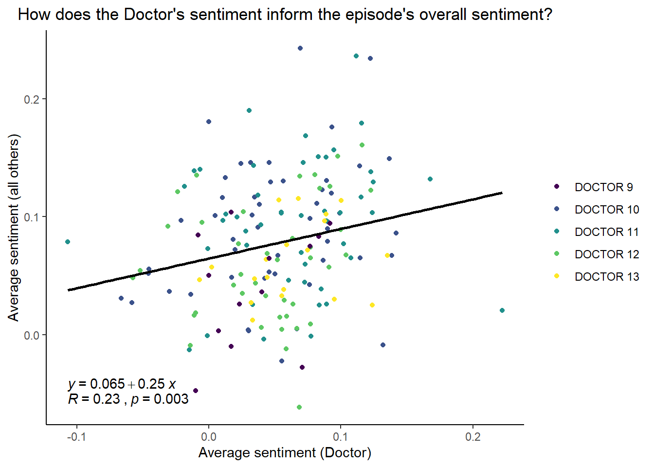
The relationship between between the average sentiment of the Doctor and that overall across episodes is quite weak; that is, the Doctor’s sentiment doesn’t track very well with the overall sentiment of the episode. This suggests that the differences in the sentiment of Doctors that we saw above are reflective of real differences in characterisation, not just differences in the tone of episodes. In general, we see that the Doctor’s overall sentiment is lower than that of other characters in a given episode.
Summary
This Doctor Who script dataset was a lot of fun to play around with and to practice my scraping skills. My analysis here has been very exploratory, but this dataset could also be used to answer specific questions about the show.
Resources
- You can find the website I scraped the scripts from here.
- I discovered another analysis of Doctor Who scripts while I was in the late stages of writing up this post. This analysis by Jean-Michel D tackles different questions than I do here, so the two posts complement each other quite well.
- Debbie Liske’s three-part tutorial on using NLP to analyse the lyrics of Prince’s music is a great read and gave me a lot of ideas on the kinds of questions you can use NLP to answer
- Although I didn’t use the
tidytextpackage, I did consult Text Mining with R by Julia Silge and David Robinson a lot for background on text mining and NLP. This is a fantastic resource. - The Quanteda tutorials site walks through many example of text analysis using
quanteda. - I found this tutorial about
igraphby Katya Ognyanova extremely useful as I was figuring outigraph. - You can find the script I used to scrape and clean the Doctor Who script data on Gitlab here.